AI Observability for Startups: 3 Key Metrics to Monitor First

Introduction
"The AI model we put into production—actually, no one is watching it." This situation is not uncommon at startups in the early stages of AI adoption. In organizations with 10 to 50 employees that have just deployed a model to production, CTOs and tech leads often struggle to decide what to prioritize monitoring with limited staff and budget. AI Observability is the framework for continuously visualizing model and system behavior through logs, metrics, and traces, enabling early detection of accuracy degradation and anomalies—but trying to set everything up at once tends to bring progress to a halt.
So, with limited resources, where should you start? This article narrows the focus to three metrics—model accuracy degradation, inference latency and error rate, and input data anomalies—and explains a minimal-configuration implementation approach using open-source tools, along with an expansion roadmap aligned with business growth.
【Hypothetical Example】One department aggregated LLM API calls tagged by department over a 90-day period, reducing the work time spent on month-end billing reconciliation by 40%. The premise was that "department codes are attached to all requests," and the setup involved simply adding a single tag column to the existing logging infrastructure.
AI Observability is not an extension of conventional monitoring but a framework for capturing model-specific degradation. Tracking only traditional metrics such as CPU usage, response time, and error rate will not reveal a quiet decline in model accuracy or qualitative shifts in input data. It is not uncommon for a system to appear to be running normally while only the model's output gradually drifts—and this is the pitfall unique to AI.
In the startup environment, with limited engineering resources, it's necessary to first decide "what to monitor, and to what extent." Trying to set everything up at once can consume weeks on initial construction alone, cutting into the development speed that matters most. Since system monitoring and model monitoring differ both in purpose and in what they observe, lining up metrics from both without distinguishing between them tends to leave both half-baked. This is precisely why narrowing down metrics and adopting a phased rollout suits startups. In the next section, we'll concretely organize this distinction and the thinking behind implementation.
Differences Between AI Observability and Traditional System Monitoring
CPU usage and response time are sufficient for checking whether a conventional system is running normally, but a different set of metrics is needed to check whether the model's judgments themselves are correct. Traditional health monitoring tracks whether the server is down or whether the API is responding within the expected time—it's a mechanism for confirming "is it running." AI Observability, on the other hand, confirms "is it running correctly," and its scope of observation extends to the quality of model output and changes in input data trends.
Even if the inference server's latency stays within the normal range, prediction accuracy can quietly decline if the input distribution in production drifts from that of training. This phenomenon cannot be detected through conventional health monitoring or error logs. NIST AI RMF's MEASURE 2.4 also calls for continuously monitoring a model's functionality and behavior after deployment, indicating that the very object of observation differs from traditional infrastructure monitoring.
In other words, the two are not substitutes but complements. Infrastructure health is covered by conventional monitoring, and the quality of the model's judgments is covered by AI Observability. In practice, the most reasonable approach is to expand the existing monitoring infrastructure by adding model-specific metrics.
Why Startups Need a Phased Approach to Adoption
If a startup aims from the outset for enterprise-grade AI Observability, it will exhaust its limited engineering resources just building the monitoring infrastructure. During the phase of exploring PMF, the model architecture and use cases themselves tend to change on a weekly basis, so designing a broad set of monitoring items from the start often means the premises collapse and the work has to be redone. Monitoring spread across all directions is like buying furniture in advance for a pivot that will render it unused.
On the other hand, proceeding to production without setting up any monitoring at all risks failing to notice accuracy degradation or increased errors until the impact on users has already grown large. If you run with zero monitoring and only learn of accuracy degradation through customer inquiries, the cost of restoring trust will exceed the cost of building the monitoring infrastructure. The real question is not "what to measure" but "what is worth measuring at the current phase"—a matter of prioritization. A realistic approach is to initially narrow the focus to high-impact metrics such as model accuracy, latency, and error rate, then add metrics like data quality as the team and data volume grow.
NIST AI RMF also calls for continuous monitoring under its MEASURE-related functions, but this should be read as grounds for clarifying priorities within a limited investment. A phased rollout is not about cutting corners on monitoring—it is precisely the decision to concentrate resources on the highest-risk areas at any given point in time.
3 Key Metrics Startups Should Monitor First

If asked what to prioritize monitoring with limited resources, the first thing to name is model accuracy degradation. Even when predictions begin to drift, the business system's alarms won't sound. Even if sales forecasts miss reality by 30%, the system logs will show no error whatsoever. This "silent degradation" is precisely what makes it troublesome—left unaddressed, it tends to lead to a situation where you only notice it after the impact on users has already spread gradually. That is exactly why, even with limited resources, accuracy monitoring should be the first place budget and manpower are allocated.
Inference latency and error rate are directly tied to whether the system is alive or dead, which makes detection itself relatively easy—but if the thresholds are set incorrectly, false alarms will proliferate and exhaust the team.
Input data anomalies often appear as a precursor to the two issues above, and while their priority is lower than accuracy degradation, they serve a role as an early warning network.
NIST AI RMF's MEASURE-related items, as well as Azure Machine Learning and SageMaker Model Monitor, all commonly list these three as monitoring categories. At the startup stage, where both manpower and budget are limited, narrowing the initial investment to these three metrics is a realistic choice.
Metric 1: Detecting Model Drift
Judgment criterion: Divide monitoring methods by the timing of ground-truth label acquisition
For tasks where ground-truth labels are obtained with a delay (such as fraud detection or demand forecasting AI), actual accuracy cannot be measured immediately. In such cases, using changes in the distribution of predicted values itself as a proxy metric is a practical approach. The prediction drift monitoring signal cited by Azure Machine Learning is based on this idea.
On the other hand, for tasks where ground-truth labels are obtained relatively quickly, model quality metrics such as accuracy and recall can be tracked directly. The reason SageMaker Model Monitor includes Model quality as a monitoring category is that it assumes operations where label acquisition is feasible.
Among the three metrics, this is the one to address first. If accuracy degradation goes unnoticed for weeks of operation, no amount of investment in the other two metrics will matter. Cases can occur where the distribution of predicted values hasn't changed, yet the decision criteria used on the ground have simply become outdated.
In the early stages, recording the mean and variance of predicted values weekly, and checking changes in feature attribution monthly, are both easy to implement. Both can be started with about the effort of adding an extra panel to a dashboard.
This is an operational approach aligned with what NIST AI RMF's MEASURE 3.1 calls "periodic tracking of known and emerging risks." For operations where label acquisition is delayed, a design that starts with proxy metrics and switches to direct accuracy metrics once labels become available is well suited.
Metric 2: Inference Latency and System Error Rate
When input token counts spike, latency worsens; when external API or GPU resource limits are hit, error rates spike—the causes behind the two differ. Many teams consider latency a higher priority than accuracy degradation, and there is a tendency for user drop-off to visibly increase once response times exceed 3 seconds.
It's easy to assume that tracking average latency alone is sufficient at first, but what actually needs to be watched is the tail of the distribution—that is, p95 and p99. It is not uncommon for p99 to exceed 15 seconds even when the average is 1.2 seconds, and this is the real cause behind the phenomenon of "the dashboard looks healthy, yet inquiries keep increasing." The reason NIST AI RMF's MEASURE 2.6 positions real-time monitoring of response time as a safety metric is precisely that averages alone fail to capture the actual situation.
Error rate also cannot be adequately captured through simple aggregation of HTTP status codes. Recording rate limiting, context window overflows, and external tool call failures separately makes it easier to distinguish whether the bottleneck lies in GPU shortage or API design issues. For details, refer to Latency Budgeting for AI Agents.
Metric 3: Detecting Input Data Anomalies (Data Drift)
Anomaly detection for input data (Data Drift) is monitoring that captures the phenomenon where the statistical tendencies of production data diverge from the data at training time. While accuracy degradation is a lagging indicator that appears as a result, data drift differs in that it can be detected in advance as a precursor. Changes in the user base, changes in external API specifications, and shifts in traffic ratios due to seasonality or campaigns often appear in log statistics before accuracy actually drops. Among the three metrics, this is the one most often deprioritized, yet it is the only monitoring approach that allows you to act preemptively.
Google Cloud's official documentation distinguishes between skew—the distributional difference between training time and inference time—and drift, which arises over time, and recommends a method of identifying the primary cause of drift using feature importance. Since few startups have the capacity to monitor all features equally, a design that narrows the focus to a handful of top features directly tied to decision-making—such as annual income or usage history for a credit score—is more operationally feasible.
The monitoring method should vary depending on the type of input. For high-dimensional data such as text or images, summary statistics alone make it difficult to capture anomalies, and situations arise where distance metrics in embedding space are used as a supplementary tool. If the data is centered on numerical values or a small number of categorical variables, tracking trends in mean, variance, and missing-rate is sufficient for the initial stage. If in doubt, start with the latter approach and add distance metrics once dissatisfaction with accuracy emerges.
Minimal-Investment Tool Stack (Comparison Table)

With limited budget and resources, are you unsure which tool to start with? If you already have operational experience with existing infrastructure, it's practical to center on Prometheus and Grafana; if you don't yet have a log collection mechanism in place, a realistic order is to first unify the output of traces and metrics with OpenTelemetry before choosing a visualization layer.
| Comparison Target | Evaluation Axis | Decision Point |
|---|---|---|
| Prometheus + Grafana | Metrics collection & visualization | If already used for server monitoring, the learning cost of adding latency and error rate is low |
| OpenTelemetry | Log/trace integration | If a monitoring mechanism isn't yet established, unify the output here first |
| MLflow | Model accuracy & experiment management | If you want to compare training-time accuracy metrics against production accuracy degradation judgments, you can reuse existing experiment records |
| Cloud-standard monitoring (Azure Machine Learning / SageMaker Model Monitor) | Data quality & drift detection | Effective if you're already training and inferring on that cloud and want to avoid additional effort |
While cloud-standard features get you up and running quickly, they offer less freedom in monitoring logic. If you're anticipating a move to multi-cloud or an in-house data center, prioritizing a highly portable Prometheus setup will keep switching costs lower. If getting something running immediately is the top priority, starting with cloud-standard features is also fine.
Criteria for Selecting Open-Source Tools
The basic approach is to choose based on integration cost with existing infrastructure. Choosing based on the sheer number of features is not uncommon to result in a tool that operators can't fully utilize and end up abandoning.
If Prometheus is already used for server monitoring, layering AI Observability on top of it keeps the learning cost lower. For small teams, the frequency of documentation updates and the speed of response to Issues can be the lifeline for handling trouble—this shouldn't be overlooked. Even if you start by only watching the three metrics of model accuracy degradation, latency, and error rate, it's worth checking whether the design allows data quality metrics to be added later.
The order of implementation also affects outcomes. If you introduce a dashboard tool first while the log collection mechanism is still unorganized, you'll later face the extra work of re-aligning trace granularity. Unifying the format of metrics and traces first with OpenTelemetry, then choosing the visualization layer afterward, results in less rework. Be sure to check license terms and commercial-use restrictions in the official documentation.
Recommended Tool Combination for Early Stages
If existing infrastructure is already running in a containerized environment, the combination of Prometheus and Grafana serves as a natural starting point; if no monitoring infrastructure exists yet, starting with log collection makes it easier to get going. Prometheus excels at collecting and storing numerical metrics, allowing inference latency and error rates to be accumulated as time series. Grafana functions as the dashboard layer that visualizes that data, making it easier to notice visual changes when thresholds are exceeded.
For detecting model accuracy degradation, rather than writing dedicated statistical processing, a configuration that periodically calculates the difference between inference results and labeled data in a batch job and exports the aggregated values to Prometheus keeps implementation costs lower. Similarly, for data anomaly detection, calculating distribution statistics of input data with a lightweight script and feeding it into the existing metrics infrastructure gets things running faster than learning a separate dedicated tool.
Note that both Prometheus and Grafana are open source, and it is advisable to check the official documentation for license terms and detailed feature information. Settling on "what to measure" before adding more tools results in fewer design changes when expanding later. This configuration is based on the judgment criterion of first centering on tools that the infrastructure operations team is already familiar with.
Implementation Steps for Initial Adoption

Once the tool configuration is decided, actual implementation can proceed in three steps. Starting with building the log collection mechanism, then visualizing it on a dashboard, and finally connecting it to alert operations—this sequence is an approachable flow for teams with limited resources.
Step 1: Building a Log and Metrics Collection System
What should be collected, and from where, to form the foundation of monitoring?
The first thing to organize is a mechanism for structuring and retaining input, output, latency, and error information as logs for each inference request. Rather than embedding this into existing application logs, inserting a wrapper process for metrics collection before and after inference calls—and recording the model version and request ID along with it—makes subsequent drift analysis and error root-cause identification easier.
Opinions diverge on the design of the collection destination. If you are already using a framework capable of outputting Prometheus-format metrics, adding inference-related custom metrics to the existing exporter involves less rework. On the other hand, if you want the flexibility to change aggregation axes later using a log-based approach, first accumulating structured logs in JSON format and building an aggregation pipeline as needed keeps initial design costs lower.
Note that when storing input data itself for the long term, it is necessary to check in advance whether it contains personal or confidential information. Detailed implementation examples for the logging infrastructure are also explained in Integrated Management of LLM Inference Logs, which can serve as a reference when considering visualization in production environments.
Step 2: Building Dashboards and Setting Thresholds
Judgment criterion: A dashboard should not simply be "looked at and left there"—it only becomes useful for monitoring once linked with thresholds.
Start with a configuration that arranges the three collected metrics—accuracy degradation, latency, and error rate—on a single screen. In Grafana, specifying Prometheus as the data source and overlaying a time-series graph with a threshold line on each panel allows you to grasp both the trend of the values and any deviation from the acceptable range at the same time.
When setting thresholds, placing arbitrary fixed values from the start without any basis tends to cause over-detection or missed detections. It is more practical to gather 1-2 weeks of baseline data after starting operations, tentatively set upper and lower bounds based on the mean and variance, and adjust them during actual operation. For example, for inference latency, check the normal response time range and agree as a team on how far a deviation from that upper bound should be considered abnormal.
Since error rate and model accuracy degradation have different characteristics, it is safer not to reuse the same threshold logic for both. Error rate is a metric where you want to detect sharp short-term spikes, whereas accuracy degradation is a metric for tracking gradual trend changes—so for the latter, smoothing out noise with a moving average before applying threshold judgment reduces false detections.
The purpose of the dashboard is "noticing anomalies," and detailed root-cause analysis is not handled here. Designing it so that deeper investigation of causes is left to subsequent alert operations or individual investigations using structured log data keeps the dashboard itself clear and easy to grasp.
Step 3: Starting Alert Operations
For metrics with high detection frequency, immediate notification is appropriate, while for metrics that change gradually, checking via daily aggregation is more suitable. The first step in alert operations is separating notification channels. Sudden changes in error rate or latency should be immediately notified via Slack, PagerDuty, and the like, while metrics that take time to judge—such as accuracy degradation or data anomalies—are more practically compiled into daily reports as email or dashboard summary notifications.
In the early stages, notifying all deviations with the same level of importance causes alerts that need attention to get buried. It is effective to operate with differentiated importance levels between cases where a threshold is simply exceeded and cases where multiple metrics deteriorate simultaneously. For example, codifying conditional branching rules—such as treating a temporary spike in latency alone as a warning level, but treating a simultaneous rise in error rate and deterioration in latency as an urgent response—can reduce the judgment burden on personnel in charge.
It is also essential to clearly designate the first responder when an alert occurs. For small teams, operating a rotation or on-call system on a weekly basis is practical. Since false detections tend to occur frequently right after operations begin, it is important to record the relationship between notification content and actual incidents during the first few weeks and reflect this in revising thresholds and rules.
Phased Expansion Roadmap

Once operation of the 3 metrics has stabilized, the next step is monitoring data quality and user impact. The 3 metrics represent only the minimum layer for observing the basic health of the model and system, and as the business grows, a deeper layer of monitoring becomes necessary.
Guidelines for expansion can be organized according to the team's growth phase as follows.
| Phase | Monitoring Target | Purpose |
|---|---|---|
| Phase 1 (Early Adoption) | Accuracy degradation, latency, error rate | Maintain the basic health of the model and system |
| Phase 2 (Around PMF) | Data quality, input data bias, user impact | Understand decision-making quality and impact on customer experience |
| Phase 3 (Expansion Phase) | Audit logs, explainability, fairness by user attribute | Establish governance structure and accountability |
Before reaching PMF (Product-Market Fit), Phase 1 alone is sufficient. However, once paying customers increase and the scope of automated decision-making expands, postponing Phase 2 data quality monitoring tends to allow bias to accumulate.
In Phase 3, internal AI governance structures and monitoring operations need to be integrated, and it is effective to consider this alongside the governance framework discussed in What is AI Governance? A Practical Guide from EU AI Act Compliance to Internal Rule Development.
If you rush and reverse this order of expansion, you tend to end up with more metrics that nobody actually looks at. For startups with limited personnel, the realistic order is to first confirm a structure capable of stably operating the 3 metrics, and only then invest in the next layer.
FAQ: AI Observability Adoption for Startups

This section answers questions commonly raised by startup personnel, such as implementation timeframes, comparisons with existing tools, and monitoring frequency. Use this to resolve pre-implementation doubts and as material for deciding your next action.
How Long Does It Take to Implement AI Observability
Decision criteria: Implementation timeframe varies depending on the team's structure and how narrowly the scope is defined.
For a minimal setup limited to the 3 metrics—model accuracy degradation, latency, and error rate—assuming a combination of an existing log collection infrastructure and open-source monitoring tools, it is feasible to launch the initial dashboard and alert operations within a few weeks. If a metrics collection mechanism is already running on the application side, it may only be necessary to add model-related metrics, which can shorten the timeframe even further in some cases.
Short answer: "Yes," if the conditions are met. "No," if the prerequisites (measurement units, tagging) are not in place.
Are Existing Monitoring Tools Not Sufficient
If you have already implemented traditional infrastructure monitoring, monitoring CPU, memory, and response time may seem sufficient, but if there is no mechanism to evaluate the model's inference results themselves, this is insufficient as AI Observability. Existing APM (Application Performance Monitoring) tools show whether the system is running normally, but cannot detect a situation where the model continues to return incorrect predictions. Any team that has faced a situation of "latency and error rate are both normal, yet inquiries from users are somehow increasing" should keenly understand this gap.
The decision point lies in whether the monitoring target is "system survival" or "model validity." Monitoring at the system level alone is sufficient only for use cases where the model's output is fixed and changes little. On the other hand, for use cases where training data or input distribution continuously changes, model-level metrics that capture accuracy degradation and data drift are essential.
A realistic approach is to expand your existing monitoring infrastructure by adding model-related metrics via Prometheus or Grafana. There is no need to rebuild from scratch—the idea of building model metrics on top of existing infrastructure is compatible with minimal-investment implementation.
Decision tree: For small scale (under 10,000 requests/month), choose spreadsheet monitoring; for medium scale, choose daily batch evaluation; for large scale (over 1 million requests/month), choose streaming evaluation. First branch based on output volume and availability of reference data, and retain only the path whose operational load is acceptable.
How Often Should Monitoring Metrics Be Checked After Implementation
Monitoring frequency branches depending on the nature of the metric. Latency and error rate require high real-time responsiveness, so it is desirable to combine always-on dashboard visualization with alerts to enable detection within minutes of an anomaly occurring. On the other hand, model accuracy degradation and data drift are difficult to observe changes in over a short period, so it is more practical to track trends through daily to weekly batch aggregation.
The decision criterion is "the time it takes for business impact to appear." Latency degradation immediately affects user experience, whereas accuracy degradation often takes days to weeks to surface, so there is no need to align the check frequency for both. In the initial stage, a two-tiered approach is likely to work well: the whole team checks the dashboard weekly, with immediate response only when a threshold is exceeded. NIST AI RMF's MEASURE 2.4 calls for continuous monitoring of functionality and behavior during production operation, and the design of frequency should also be reviewed according to the magnitude of the risk.
As the number of users and the frequency of model updates increase, the check cycle should be shortened. At the PoC stage, when traffic is low, weekly checks may be sufficient.
Step-by-step:
- Sample output quality for one week to establish a baseline.
- Fix the monitoring metrics and thresholds in a document.
- Determine the escalation destination for when a threshold is breached.
- Review the false-positive rate weekly and update the thresholds.
Establishing operations in this order makes it easier to prevent delays in detecting quality degradation. When in doubt, start testing with the path that has the smallest scope of impact.
Author & Supervisor

Yusuke Ishihara
Started programming at age 13 with MSX. After graduating from Musashi University, worked on large-scale system development including airline core systems and Japan's first Windows server hosting/VPS infrastructure. Co-founded Site Engine Inc. in 2008. Founded Unimon Inc. in 2010 and Enison Inc. in 2025, leading development of business systems, NLP, and platform solutions. Currently focuses on product development and AI/DX initiatives leveraging generative AI and large language models (LLMs).
Recommended Articles


Terms related to this article
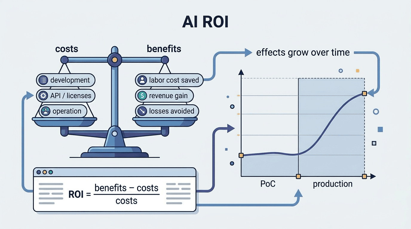
AI ROI (Return on Investment in AI)
AI ROI is a metric that quantitatively measures the effects obtained — such as operational efficienc

AI Ready
"AI Ready" is a concept that refers to the state in which a company is fully prepared to immediately

Predictive Maintenance
Predictive maintenance is a method that uses AI to analyze sensor data and operation logs, predictin