Implementing AI Observability: Integration with Existing Application Monitoring and Phased Adoption

Why Integrating Existing Application Monitoring with AI Observability Matters

Existing monitoring infrastructure holds valuable assets in the form of metrics and alert configurations accumulated over many years. As AI systems are introduced, completely discarding and replacing these assets all at once is not practical. This article explains how to gradually integrate AI Observability while making the most of existing assets.
Existing monitoring infrastructure contains metrics, logs, and traces that have been accumulated over many years. These are not "old data" — they are valuable baselines for evaluating the behavior of AI systems.
Infrastructure metrics (CPU usage, memory, latency) directly correlate with the inference load of AI models. Discarding data already collected by existing Prometheus or Datadog instances and rebuilding from scratch is like redrawing a map from a blank sheet while already holding one. Leveraging reusable assets is the most direct path to keeping implementation costs down.
The following are specific examples of existing data that can be put to use:
- Infrastructure metrics: Can be repurposed for anomaly detection of GPU/CPU load during model inference
- Application logs: Serve as a foundation for linking request/response pairs to AI input/output traces
- Distributed traces: Model calls can be added as spans to existing tracing pipelines (Jaeger, Zipkin, etc.)
- Alert rules: Threshold-based alerts can be operated in parallel with AI Observability anomaly detection
AI-specific metrics monitored by Amazon SageMaker Model Monitor — such as Data quality and Model quality — can also be stored in the same storage layer as existing metrics collection infrastructure.
Why Gradual Integration Is More Practical Than a Full Replacement
Many teams think, "Let's first overhaul all existing monitoring tools, then introduce AI Observability." In practice, however, a wholesale replacement tends to create the risk of zero visibility during the migration period, often causing a temporary loss of incident response capability. A gradual integration approach allows teams to steadily build capabilities while maintaining operational stability.
There are three main reasons why gradual integration is the more realistic choice:
- Protecting existing assets: Dashboards, alert rules, and SLO configurations accumulated in Prometheus, Datadog, Grafana, and similar tools represent knowledge assets that teams have refined over a long period. A wholesale migration risks losing these assets and incurring reconstruction costs.
- Localizing risk: AI model monitoring requirements — such as hallucination rate, latency distribution, and drift detection — differ from traditional infrastructure monitoring. Running old and new monitoring layers in parallel allows the blast radius of any issues to be contained to AI-related components only.
- Distributing the learning curve: It takes time for SRE teams to acquire concepts specific to AI Observability. Dividing the work into phases allows skills to be built up incrementally while continuing operations.
A phased approach is also advantageous from a budget perspective. The results of effectiveness measurements obtained in each phase can be used to inform investment decisions for the next phase, making it easier to maintain accountability to management.
That said, gradual integration does come with its own caveats.
Designing the Integration Architecture: A Three-Layer Structure

The integration architecture consists of three layers: normalization of existing monitoring data, an AI-dedicated pipeline, and unified analytics. By keeping each layer independent, AI Observability can be added incrementally without interrupting existing tools.
Layer 1: Normalizing and Aggregating Existing Monitoring Data
Have you ever wondered whether existing Prometheus metrics or Elasticsearch logs could be used as-is for AI monitoring? Unfortunately, in many environments, monitoring tools each use different data formats, making it impossible to connect them directly to an AI Observability analytics platform. The role of the first layer is to normalize this heterogeneous data into a unified schema, putting it into a form that downstream pipelines can readily work with.
There are three main categories of data subject to normalization:
| Data Type | Typical Sources | Key Normalization Points |
|---|---|---|
| Metrics | Prometheus, Datadog, CloudWatch | Unifying timestamps to UTC, standardizing units (ms/s, etc.) |
| Logs | Elasticsearch, Splunk, Fluentd | Converting to structured JSON, unifying log levels (INFO/WARN/ERROR) |
| Traces | Jaeger, Zipkin, OpenTelemetry | Standardizing span ID and trace ID formats, organizing service name namespaces |
For implementing normalization, a practical approach is to deploy an OpenTelemetry Collector as a gateway. It receives data from each existing tool, converts it to OTLP (OpenTelemetry Protocol) format, and forwards it downstream. Since this requires minimal changes to existing Prometheus exporters or Fluentd pipelines, it can be introduced without interrupting current monitoring operations.
Layer 2: Data Pipeline for AI Observability
Data normalized in Layer 1 is, so to speak, "source text translated into a common language." In Layer 2, we build a dedicated pipeline for interpreting that source text within the context specific to AI systems.
The core of Layer 2 is a processing system that collects and transforms AI-specific signals generated by LLMs and ML models. Concretely, it handles the following four types of data streams:
- Inference logs: Prompt-response pairs, token counts, latency
- Model metrics: Prediction confidence scores, hallucination detection flags, drift indicators (Jensen-Shannon Distance, Population Stability Index, etc.)
- Feature store input distributions: Differences between feature statistics at inference time and the training-time distribution
- Context traces: Records of retrieval sources and referenced chunks in RAG pipelines
A key implementation decision is choosing between push and pull patterns. Signals requiring real-time delivery—such as inference logs—should be pushed via an event stream (e.g., Kafka or Kinesis), while signals for which batch computation is sufficient—such as drift indicators—are better suited to a pull design using scheduled jobs.
A common pitfall for teams accustomed to existing APM tools or Prometheus is attempting to treat all AI signals as metrics. Prompt-response pairs are text data and require different storage and retrieval interfaces than time-series metrics.
Layer 3: Unified Analysis and Anomaly Detection
Layer 3 receives the data prepared in Layers 1 and 2, performing cross-cutting analysis across existing application monitoring and AI-specific signals to detect anomalies at an early stage.
It is tempting to assume that "simply applying existing threshold-based alerts to AI metrics as-is will be sufficient." In practice, however, LLM latency and hallucination rates often do not follow a normal distribution, causing static thresholds to produce frequent missed detections and false positives. An approach that combines statistical change-point detection with anomaly scoring tends to be more effective.
Concretely, the following three analytical capabilities are consolidated into a unified dashboard:
Implementation Steps for Building the Data Pipeline

To make the three-layer architecture work in practice, the flow of data must be implemented as a concrete sequence of steps. The process proceeds in four steps: extracting data from existing tools, normalizing it, extending it for AI Observability, and storing it in unified storage.
Step 1: Extracting Data from Existing Monitoring Tools
"How do we actually pull data out of our existing Prometheus or Datadog?"—this is a question that stops many teams in their tracks at the very start of an integration project.
The starting point for data extraction is taking stock of the export capabilities offered by the monitoring tools currently in operation. The extraction methods for major tools are as follows:
| Tool | Primary Extraction Method | Data Types Available |
|---|---|---|
| Prometheus | Remote Write / HTTP API | Metrics (time-series) |
| Datadog | Metrics API / Log Forwarding | Metrics, Logs |
| Grafana Loki | LogQL HTTP API | Logs |
| Jaeger / Zipkin | gRPC / HTTP Collector | Distributed Traces |
| ELK Stack | Logstash Output / Elasticsearch API | Logs, Metrics |
The first thing to verify at extraction time is sampling rate and timestamp precision. If you attempt to retroactively correlate metrics that an existing system has aggregated at fixed intervals with AI model inference latency (measured in milliseconds), the differing time-series granularities will prevent correlation analysis from working correctly. Normalizing timestamps to UTC at the extraction stage and retaining the original granularity as metadata will significantly simplify downstream normalization.
A second point requiring attention is log cardinality explosion.
Step 2: Normalizing Metrics, Logs, and Traces
Data collected from different monitoring tools varies in format, units, and timestamp precision. This is analogous to multiple speakers of different dialects participating in the same meeting—without agreeing on a common language, the discussion cannot cohere. Normalization is the process of defining that "common language."
Metric normalization begins with unifying units and granularity. Because Prometheus may return second-based counters while CloudWatch returns millisecond-based gauges, timestamps should be aligned to UTC ISO 8601 format and sampling intervals standardized to either 60 or 30 seconds. Label name inconsistencies—such as host versus hostname—should also be resolved and normalized to a shared key set (service, env, region).
Log normalization requires handling structured logs (JSON) and unstructured logs (plain text) separately. Unstructured logs should have fields extracted via regular expressions or parsers and converted into a common schema containing at minimum timestamp, severity, message, and trace_id. For older logs that lack a trace_id, a pseudo-ID can be generated from the service name and timestamp and assigned to them, enabling trace joins in subsequent processing.
Trace normalization is most practically achieved by adopting the OpenTelemetry Trace Context specification (W3C traceparent header) as the standard baseline.
Step 3: Adding Extended Fields for AI Observability
This step enriches normalized metrics and logs with AI-specific contextual information. It is tempting to assume that reusing existing fields will suffice, but in practice, designing dedicated extension fields for tracking model behavior significantly improves the efficiency of subsequent anomaly detection and root cause analysis.
Extension fields to add can be broadly classified into three categories.
Model Identification & Version Management
model_id: Identifier for the model currently deployedmodel_version: Essential for comparisons during A/B testing and staged rolloutsserving_endpoint: Used for correlation in environments where multiple endpoints run in parallel
Inference Quality & Performance
latency_p99: For understanding tail latency (relying on averages alone causes outliers to be missed)token_count_input/token_count_output: The foundation for cost management and throttling decisionsconfidence_score: The confidence level output by the model. Functions as a supplementary indicator for hallucination detection
Data Drift Detection
feature_hash: A hash of the input features. Used to verify reproducibility of identical requestsprediction_label: The label of the inference result.
Step 4: Storing Data in Unified Storage
This is the stage where normalized and enriched data is stored in the appropriate storage destination for its intended purpose. Design decisions made here directly affect the speed and cost of downstream analysis.
The basic principle is to select storage destinations based on the nature of the data. For real-time alerting use cases, writing to a time-series database (such as Prometheus or InfluxDB) is appropriate, while long-term drift analysis and batch aggregation are better suited to object storage (S3-compatible) or a data warehouse. When both use cases coexist, adopting a two-tier architecture that separates the hot path from the cold path allows query performance and storage costs to be balanced simultaneously.
An important implementation consideration is schema version management. AI Observability-specific extension fields (e.g., model_version, prompt_token_count, drift_score) are added retroactively to existing monitoring schemas, so the design must maintain backward compatibility to prevent schema changes from breaking existing dashboards and alerts. Leveraging a schema registry such as Apache Avro or Protocol Buffers enables automated compatibility checks when fields are added.
Write idempotency is another easily overlooked point. To prevent duplicate data from being introduced during pipeline reprocessing or retries, it is recommended to incorporate either upsert operations keyed on an event ID or a pre-write deduplication check.
Phased Adoption Strategy: A Three-Phase Approach

A practical approach to adopting AI Observability is to proceed in three phases: pilot, partial integration, and full production operation. By defining clear success criteria for each phase and making the transition decision to the next phase based on quantitative measures, the monitoring scope can be expanded incrementally while keeping risk under control.
Phase 1: Pilot Deployment (Months 1–2)
The pilot phase is about "starting small and learning" before rolling out to the entire system. Just as clinical trials are conducted before administering a new drug to all patients, AI Observability should also be validated within a limited scope before being expanded.
Narrowing the Target Scope
For the first one to two months, focus on a single AI service or one inference endpoint. The selection criteria are the following three points:
- Moderate traffic volume (neither overloaded nor idle)
- An existing APM agent is already running
- Business impact in the event of a failure is limited and rollback is straightforward
Minimum Set of Measurements
It is important to keep the metrics collected during the pilot period focused. In addition to the existing "golden signals" of latency, error rate, and throughput, add three AI-specific indicators: token consumption, hallucination detection rate, and the latency distribution of prompt responses. At this stage, prioritize "making differences visible when placed alongside existing dashboards" over comprehensiveness.
Pre-defining Success Criteria
Set numerical targets before starting so that a "go or no-go" decision can be made at the end of the phase. Examples include: "Keep the false positive rate of AI-specific alerts at or below the false positive rate of existing alerts" and "Keep the additional pipeline latency within 50ms at P99." Proceeding without clear targets means the decision to move to Phase 2 will rely on intuition, so caution is warranted.
Team Structure
Operate with a small team of one to two SREs and one ML engineer.
Phase 2: Partial Integration (Months 2–4)
This phase uses the insights gained during the Phase 1 pilot to gradually expand monitoring coverage to multiple services in the production environment.
It is tempting to think that "if it was proven in the pilot, the remaining services can all be rolled out at once." In practice, however, data formats and update frequencies differ from service to service, causing exceptions in normalization rules to accumulate, making a bulk rollout a breeding ground for quality issues. Adding services two or three at a time in order of priority makes isolating and resolving problems significantly easier.
The main tasks to address in this phase are as follows:
- Expanding target services: Prioritize based on traffic volume and business impact, and roll out starting with services that incorporate AI models
- Generalizing normalization rules: Templatize the data transformation logic that was handled on a case-by-case basis during the pilot to reduce the cost of onboarding new services
- Refining alert rules: In addition to existing threshold-based alerts, add AI-specific indicators such as hallucination rate and drift detection as alerting conditions
- Establishing a cross-team review cadence: Establish a weekly cycle in which SREs, ML engineers, and product owners review metrics together
As the completion criteria for this phase, confirm that the majority of production traffic for the target services is flowing through the integrated pipeline and that there is no impact on existing dashboards. Defining completion criteria numerically enables an objective decision to be made regarding the transition to Phase 3.
Phase 3: Transition to Full Production (Months 4–6)
For systems whose integrations have stabilized in Phase 2, proceed with the transition to full production operations. The core of this stage is the transfer of monitoring responsibility. Formally incorporate the AI observability dashboards and alerts into the SRE team's primary response flow.
Whether to proceed with the transition is determined by the achievement status of the SLOs (Service Level Objectives) defined in Phase 2. A practical decision framework is to transition systems that are consistently meeting their SLOs to full production, while maintaining the Phase 2 monitoring setup for systems that remain unstable.
The main tasks to be carried out at the time of transitioning to full production are as follows:
- Runbook preparation: Document incident response procedures for AI-specific alerts, such as sudden spikes in hallucination rate and data drift detection.
- On-call integration: Add AI model anomalies to the existing on-call rotation and conduct training so that the responsible personnel can respond appropriately.
- Automated retraining pipeline integration: Connect the model retraining workflow triggered by drift detection with the existing CI/CD pipeline.
- Cost optimization: Based on the metrics collected in Phase 2, adjust excessive log collection and sampling rates to optimize operational costs.
Even after the transition, it is recommended to allow a parallel operation period of 2–4 weeks alongside existing monitoring tools (Prometheus, Datadog, etc.). Only after confirming that alerts from the AI observability side demonstrate detection accuracy equivalent to existing tools should the legacy alert rules be gradually disabled.
Coexisting with Legacy Systems: Implementation Considerations

In almost no case can the existing monitoring infrastructure be immediately decommissioned after introducing AI Observability. This section organizes the implementation considerations for safely navigating the coexistence period from three perspectives: continued operation of alerts and dashboards, data duplication for fallback, and mitigating performance impact.
Maintaining Existing Alerts and Dashboards
Existing alerts and dashboards are, so to speak, a "field map" refined through years of operation. When introducing AI Observability, it is not advisable to wipe this map clean and start from scratch.
The basic policy is to continue operating existing Grafana dashboards and PagerDuty alerts as-is, while adding AI-specific metrics (hallucination rate, token consumption, latency distribution, etc.). Keep the following three points in mind:
- Alert coexistence configuration: Without modifying existing CPU, memory, and error rate alert rules, add AI-specific alerts (e.g., inference latency exceeding a threshold, sudden drop in model quality score) on a separate channel or with a separate tag.
- Dashboard extension: Rather than deleting existing panels, add new panels to the bottom of the same dashboard or in a separate tab. In Grafana, simply switching the
datasourceallows you to display the AI Observability data source in parallel. - On-call continuity: Until dedicated personnel for AI-related alerts are assigned, add AI alerts to the existing on-call rotation to maintain a state where the SRE team can handle initial response.
One notable exception to be aware of: AI alert thresholds may use different units than conventional infrastructure metrics. For example, a model quality score operates on a 0–1 scale, which differs in meaning from CPU utilization (%). When mixing these on the same dashboard, clearly label panel titles and units to prevent misinterpretation.
Data Duplication and Fallback Strategy
When running AI Observability infrastructure in parallel with existing monitoring, the initial instinct is often to "aggregate data in one place and then switch over." In practice, however, continuing to send data to both systems until the switchover is complete allows you to localize the impact of any failures.
With data duplication, you maintain writes to the existing monitoring storage (Prometheus, Elasticsearch, etc.) while simultaneously sending the same events to the newly established AI Observability pipeline. This configuration ensures that even if a failure occurs in the new pipeline, existing alerts continue to function, preventing any impact on SLAs.
A practical fallback strategy is designed in the following three levels:
- Level 1 (Routing switchover): Modify routing rules in the load balancer or message broker (e.g., Kafka) to immediately stop sending data to the new pipeline and consolidate traffic to the existing system.
- Level 2 (Buffering): In preparation for the new pipeline becoming temporarily unresponsive, retain up to several minutes' worth of events in a queue and resend them after recovery.
- Level 3 (Schema compatibility maintenance): Maintain a format readable by existing tools in a normalization layer, preserving a state where the same data can be referenced from either system.
If you are concerned about storage costs from duplication, an effective approach is to sample the data sent to the AI Observability side (e.g., approximately 10–20% of traces) while maintaining full collection on the existing system.
Minimizing Performance Overhead
The data collection processing of AI observability places additional load on the existing monitoring pipeline. To minimize overhead, the choice of collection method and processing timing is critical.
First, configure an appropriate sampling strategy. Synchronously collecting traces for all requests can have a noticeable impact on latency. In stable production environments, adopting probabilistic sampling (e.g., targeting 10–20% of all requests) allows you to reduce processing costs while retaining the signals necessary for anomaly detection. On the other hand, immediately after a new model release or during incident investigation, it is effective to temporarily increase the sampling rate to secure detailed traces.
Next, enforce asynchronous writes throughout. Design the system so that log and metric writes are decoupled from the critical path of request processing and sent asynchronously via a buffer queue. This ensures that even if the backend storage or analytics infrastructure experiences temporary delays, the response time of the application itself is not affected.
Narrowing down the fields collected is also effective. Extended fields required for AI observability (such as prompt token count, model latency, and hallucination detection score) tend to result in larger payloads compared to existing monitoring data. Manage fields that need to be collected continuously separately from those that are only enabled during debugging, in order to reduce data transfer volume during normal operations.
Finally, set resource limits on the collection agent side. By placing upper limits on the CPU and memory usage of collection agents, you can prevent the monitoring infrastructure from competing for resources with the host application.
ROI Measurement Framework for Investment Decisions

Quantitative metric design is essential for visualizing the ROI of AI Observability adoption. We systematically evaluate ROI along three axes: pre/post-adoption comparison metrics, cost and effectiveness measurement by phase, and criteria for continued investment decisions.
Comparing Metrics Before and After Adoption
To measure ROI, it is essential to first establish a "baseline" before adoption. Just as failing to take an initial measurement in weight management makes it impossible to see changes, monitoring metrics cannot prove improvement without a starting point.
Metrics to Record Before Adoption
| Category | Example Metrics | Measurement Method |
|---|---|---|
| Incident Response | MTTD (Mean Time to Detect) / MTTR (Mean Time to Recover) | Incident management tool logs |
| Quality | Hallucination rate / Misclassification rate | Manual review sampling |
| Operational Cost | Alert response effort (person-hours/month) | Ticket system work hours |
| Model Health | Lead time to data drift detection | Statistical logs from existing monitoring |
Secure a minimum of 4 weeks for pre-adoption measurement to obtain representative data that includes seasonal variations and weekly patterns.
Metrics to Compare After Adoption
After integrating AI Observability, re-measure using the same definitions over the same period. The three key changes to watch for are:
- Reduction in MTTD: Consolidating model quality alerts with existing infrastructure alerts into a single dashboard tends to reduce detection delays.
- Changes in false positive rate: Adding AI-specific drift detection has been reported to initially increase false positives. Quantify accuracy improvements by comparing before and after tuning.
- Changes in response effort: Once automated triage begins functioning, person-hours spent on alert response tend to decrease incrementally.
Measuring Costs and Benefits at Each Phase
Attempting to evaluate adoption costs as a single lump sum across all phases tends to make the initial investment appear large, causing decision-making to stall. In practice, changing the unit of measurement by phase is more effective for both communicating with management and driving improvement cycles on the ground.
Phase 1 (Pilot) — Units of Measurement
- Input costs: Engineer effort (person-days) + tool license trial fees
- Effectiveness metrics: Change in mean time to anomaly detection (MTTD) for the target service, change in alert false positive rate
- At this stage, prioritize qualitative evaluation of "whether detection accuracy improved" over monetary conversion, and use the results to decide whether to proceed to the next phase
Phase 2 (Partial Integration) — Units of Measurement
- Input costs: Data pipeline construction effort + additional storage costs
- Effectiveness metrics: Reduction in incident response time (MTTR), change in on-call volume
- If MTTR has decreased, converting the time saved into a monetary value based on the hourly rate of operations engineers makes it easier to use in management-level reporting
Phase 3 (Full Operation) — Units of Measurement
- Input costs: Production deployment effort + ongoing infrastructure maintenance costs
- Effectiveness metrics: Number of incidents caused by model drift, trends in SLO violation rates
- Only at this stage should you calculate the "cumulative investment-to-effect ratio across Phases 1–3" to use as a basis for continued investment decisions
It is recommended to conduct measurements not only once at the end of each phase, but also at a midpoint within the phase (4–6 weeks after the start).
Criteria for Deciding on Continued Investment
When deciding whether to transition from Phase 2 to Phase 3, or to invest in further feature expansion, a simple cost comparison is insufficient — a multi-metric decision framework is required.
The primary criteria for evaluating continued investment are as follows:
- Incident detection lead rate: If the proportion of AI model-related failures detected proactively is trending upward, this is a signal to continue investing
- Changes in alert response effort: Verify whether the false positive rate has decreased and whether average on-call response time has shortened
- Lead time from drift detection to remediation: Measure whether model quality degradation is being caught early and whether retraining or model switching is being carried out promptly
- Team proficiency: Qualitatively assess whether both SRE and ML engineers are actively using the integrated tools on a daily basis
As a decision threshold: if both detection rate and effort reduction show improvement, this provides grounds to proceed with investment in the next phase. Conversely, if costs are rising while metrics remain flat, it is advisable to first revisit the architecture or narrow the scope of coverage.
It is also important to establish fixed checkpoints for continued investment decisions. Rather than reviewing only at phase completion, it is recommended to monitor metric trends in monthly reviews and, if a sharp deterioration occurs, to bring forward the investment reassessment accordingly.
Ultimately, the essential criterion for continued investment is whether AI Observability is contributing to faster business decision-making and improved reliability.
Common Challenges and Solutions When Implementing Integration

In real-world integration deployments, three challenges repeatedly emerge: data quality inconsistencies, skill gaps between teams, and vendor lock-in. By clarifying the causes and countermeasures for each, you can prevent adoption from stalling.
Addressing Data Quality Inconsistencies
Monitoring data collected from different systems tends to be integrated with inconsistent units and granularity. This is similar to multiple speakers of different dialects talking in the same meeting room—each individual statement may be accurate, yet the whole fails to make sense.
Data quality inconsistencies manifest primarily in three patterns:
- Timestamp misalignment: Prometheus records at millisecond precision while legacy systems may record at second precision, which can cause the chronological order of events to be reversed during correlation analysis
- Metric name collisions:
latencyandresponse_timemay refer to the same concept in different systems, or conversely, identically named metrics may use different aggregation methods (p95 vs. average) - Differences in handling missing values: One system records missing values as
nullwhile another fills them with0, which can cause anomaly detection models to produce false positives
An effective countermeasure is to embed validation rules into the data normalization layer. Specifically, this means executing schema validation at ingestion time and routing records with detected inconsistencies to an isolation queue rather than allowing them into the main flow. Establish an operational cycle of periodically reviewing isolated data and updating transformation rules accordingly.
For timestamp misalignment, in addition to enforcing NTP synchronization, a practical approach is to configure a tolerance window (e.g., ±500ms) on the ingestion pipeline side and perform join processing within that window. Metric name collisions can be absorbed by maintaining a metadata catalog that defines a unified naming convention, along with a mapping table.
Closing Skill Gaps Across Teams
When addressing skill gaps, the initial instinct is often to think "everyone should catch up to the ML engineers," but in practice, dividing the knowledge to be acquired by role leads to higher retention rates.
Integrating AI observability involves three parties—SRE, DevOps, and ML engineers—making it a situation where knowledge asymmetry between teams easily generates friction. Starting from the role-based skill map below and distributing learning costs accordingly is an effective approach.
| Role | Priority Skills to Acquire | Areas to Understand Supplementarily |
|---|---|---|
| SRE | Operating drift detection alerts, threshold configuration | Understanding the meaning of model quality metrics |
| DevOps | Integrating data pipelines into CI/CD | Structure of feature stores |
| ML Engineer | Integration with existing monitoring tools (Prometheus, Grafana, etc.) | Concepts of SLOs and error budgets |
For practical retention, "joint incident response" is more effective than classroom learning. When events such as a sudden spike in hallucination rate or a drop in prediction accuracy occur in production, repeatedly running exercises where SREs and ML engineers work through root cause analysis while looking at the same dashboard naturally builds shared understanding of each other's terminology and decision-making frameworks.
For documentation, creating a "terminology cross-reference table" that maps AI-specific metrics (such as Jensen-Shannon Distance and Population Stability Index) to existing SLI/SLO terminology helps reduce misunderstandings between teams.
Avoiding Vendor Lock-In
In tool selection for AI observability, dependency on a specific vendor carries the risk of significantly increasing migration costs later. Designing to distribute dependencies across the data collection layer, storage layer, and visualization layer is key to maintaining long-term flexibility.
Concretely, keep the following three points in mind from the time of adoption:
- Adopt open-standard data formats: Conforming to the OpenTelemetry specifications for traces, metrics, and logs allows you to swap out the backend at a later stage. Embedding a collector that relies solely on a proprietary SDK will require a complete rewrite of instrumentation when switching
- Separate the storage and query layers: Retaining data via the Prometheus-compatible Remote Write API or in Parquet format allows you to carry over existing data even if you switch visualization tools from Grafana to another product
- Verify export capabilities before signing a contract: With SaaS-based AI observability products, full data export is sometimes a paid option. It is important to explicitly document the export format, frequency, and cost at the contract stage
As a decision framework for tool selection: if you want to reduce operational costs with a single vendor's integrated suite, accept the lock-in but calculate support quality and migration costs in advance; if you anticipate future multi-cloud deployment or in-house development, prioritize open-standard compliance. This distinction provides a useful basis for the decision.
ผู้เขียน・ผู้ตรวจสอบ

Yusuke Ishihara
เริ่มเขียนโปรแกรมตั้งแต่อายุ 13 ปี ด้วย MSX หลังจบการศึกษาจากมหาวิทยาลัย Musashi ได้ทำงานพัฒนาระบบขนาดใหญ่ รวมถึงระบบหลักของสายการบิน และโครงสร้าง Windows Server Hosting/VPS แห่งแรกของญี่ปุ่น ร่วมก่อตั้ง Site Engine Inc. ในปี 2008 ก่อตั้ง Unimon Inc. ในปี 2010 และ Enison Inc. ในปี 2025 นำทีมพัฒนาระบบธุรกิจ การประมวลผลภาษาธรรมชาติ และแพลตฟอร์ม ปัจจุบันมุ่งเน้นการพัฒนาผลิตภัณฑ์และการส่งเสริม AI/DX โดยใช้ generative AI และ Large Language Models (LLM)
บทความแนะนำ


คำศัพท์ที่เกี่ยวข้องกับบทความนี้

AI ออบเซอร์แวนบิลิตี้ (AI Observability)
แนวปฏิบัติในการดำเนินงานเพื่อติดตามและแสดงผลข้อมูลการทำงานของระบบ AI ที่ใช้งานจริงอย่างต่อเนื่อง ทั้
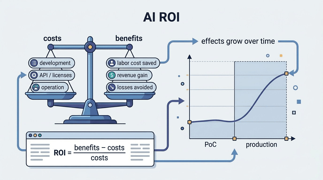
AI ROI (ผลตอบแทนจากการลงทุนด้าน AI)
AI ROI คือ ตัวชี้วัดที่ใช้วัดผลลัพธ์เชิงปริมาณของการปรับปรุงประสิทธิภาพการทำงานและการเพิ่มรายได้ที่ไ

การโจมตีห่วงโซ่อุปทาน (Supply Chain Attack)
การโจมตีผ่านห่วงโซ่อุปทาน (Supply Chain Attack) คือวิธีการโจมตีที่แทรกแซงกระบวนการพัฒนาและแจกจ่ายซอฟ